07: Combining data from multiple netcdf files

In some cases, people will choose to break down their data into multiple smaller netcdf files that they will publish in a single data collection. There are a number of good reasons to do this.

• The data user can access only the data they are interested in.

• Each file can be simpler with potentially less dimensions and less missing values. Imagine you have 10 depth profiles that all sample a different set of depths. If these profiles were included in a single netcdf file, the file would most likely a single depth dimension and coordinate variable which would need to account for all 10 depth profiles. Alternatively, 10 depth dimensions and coordinate variables could be included.

• Each individual file can be assigned a separate set of global attributes which describe the data more accurately. For example each file could have global attributes for the coordinates and timestamp. If multiple depth profiles are stored in a single file, only the minimum and maximum coordinates and timestamp can be encoded into the global attributes.

• Imagine you are looking for data in a data centre. You want to find depth profiles in a certain area of interest on a map. Files that include a single depth profile will be presented as points on the map. Files that include multiple depth profiles will be presented as a bounding box on a map, and without opening up the file it could be unclear whether the file includes data for your area of interest.

A common reaction to learning that data are divided into multiple files is that extracting the data will involve more work. However, if the files are similar (and they should be if they follow the CF and ACDD conventions) this is not neccessarily the case.

In this notebook we will look at how to combine data from multiple netcdf files into a single object (e.g. dataframe, multi-dimensional array) that you can use.

from IPython.display import YouTubeVideo
YouTubeVideo('AbLRV5YUW2g')

Introducing the data

The link below is an OPeNDAP access point to CTD data collected as part of the Nansen Legacy data. The data are grouped together by cruise and each CF-NetCDF file contains data from a single depth profile. https://opendap1.nodc.no/opendap/physics/point/cruise/nansen_legacy-single_profile/

Each file has it’s own access point like this https://opendap1.nodc.no/opendap/physics/point/cruise/nansen_legacy-single_profile/NMDC_Nansen-Legacy_PR_CT_58US_2021708/CTD_station_ISG_SVR1_-Nansen_Legacy_Cruise-_2021_Joint_Cruise_2-1.nc.html

And anyone can download some or all of the data from the CF-NetCDF file into ASCII files. This makes data access a lot easier for people who don’t yet know how to work with NetCDF files.

We can load into Python by removing the .html suffix and including the rest of the URL as our filepath. You don’t have to download the data!

import xarray as xr

xrds = xr.open_dataset('https://opendap1.nodc.no/opendap/physics/point/cruise/nansen_legacy-single_profile/NMDC_Nansen-Legacy_PR_CT_58US_2021708/CTD_station_ISG_SVR1_-_Nansen_Legacy_Cruise_-_2021_Joint_Cruise_2-1.nc')
xrds

<xarray.Dataset>
Dimensions:        (PRES: 259)
Coordinates:
  * PRES           (PRES) float32 2.0 3.0 4.0 5.0 ... 257.0 258.0 259.0 260.0
Data variables: (12/33)
    PRES_QC        (PRES) float32 ...
    TEMP           (PRES) float32 ...
    PSAL           (PRES) float32 ...
    FLU2           (PRES) float32 ...
    CNDC           (PRES) float32 ...
    DENS           (PRES) float32 ...
    ...             ...
    OXYOCPVL-1_QC  (PRES) float32 ...
    SPAR_QC        (PRES) float32 ...
    PAR_QC         (PRES) float32 ...
    PSAL-2_QC      (PRES) float32 ...
    TEMP-2_QC      (PRES) float32 ...
    ATTNZS01_QC    (PRES) float32 ...
Attributes: (12/73)
    qc_manual:                       Recommendations for in-situ data Near Re...
    contact:                         datahjelp@hi.no
    distribution_statement:          These data are public and free of charge...
    naming_authority:                no.unis
    license:                         https://creativecommons.org/licenses/by/...
    data_assembly_center:            IMR
    ...                              ...
    geospatial_vertical_resolution:  1 dbar
    pi_email:                        jannes@unis.no
    pi_institution:                  University Centre in Svalbard
    station_name:                    ISG/SVR1
    metadata_link:                   https://doi.org/10.21335/NMDC-2085836005...
    _NCProperties:                   version=2,netcdf=4.6.3,hdf5=1.10.5

xarray.Dataset

• Dimensions:
  • PRES: 259
• Coordinates: (1)
  • PRES
    (PRES)
    float32
    2.0 3.0 4.0 ... 258.0 259.0 260.0

    axis :

    Z

    uncertainty :

    comment :

    ancillary_variables :

    PRES_QC

    standard_name :

    sea_water_pressure

    long_name :

    Sea pressure

    units :

    dbar

    positive :

    down

    data_mode :

    D

    coverage_content_type :

    physicalMeasurement

    array([  2.,   3.,   4., ..., 258., 259., 260.], dtype=float32)

• Data variables: (33)
  • PRES_QC
    (PRES)
    float32
    ...

    conventions :

    Copernicus Marine In Situ reference table 2

    valid_min :

    0

    valid_max :

    9

    flag_values :

    [0 1 2 3 4 5 6 7 8 9]

    flag_meanings :

    no_qc_performed good_data probably_good_data bad_data_that_are_potentially_correctable bad_data value_changed value_below_detection nominal_value interpolated_value missing_value

    long_name :

    Sea pressure quality flag

    [259 values with dtype=float32]

  • TEMP
    (PRES)
    float32
    ...

    standard_name :

    sea_water_temperature

    long_name :

    Sea temperature

    units :

    degrees_C

    valid_min :

    -2.5

    valid_max :

    40.0

    ancillary_variables :

    TEMP_QC

    data_mode :

    D

    coverage_content_type :

    physicalMeasurement

    [259 values with dtype=float32]

  • PSAL
    (PRES)
    float32
    ...

    standard_name :

    sea_water_practical_salinity

    long_name :

    Practical salinity

    units :

    0.001

    valid_min :

    2.0

    valid_max :

    41.0

    ancillary_variables :

    PSAL_QC

    data_mode :

    D

    coverage_content_type :

    physicalMeasurement

    [259 values with dtype=float32]

  • FLU2
    (PRES)
    float32
    ...

    standard_name :

    mass_concentration_of_chlorophyll_a_in_sea_water

    long_name :

    Chlorophyll-a fluorescence

    units :

    mg m-3

    valid_min :

    0.0

    valid_max :

    100.0

    ancillary_variables :

    FLU2_QC

    data_mode :

    R

    comment :

    Fluorescence, WET Labs ECO-AFL/FL [mg/m^3]

    coverage_content_type :

    physicalMeasurement

    [259 values with dtype=float32]

  • CNDC
    (PRES)
    float32
    ...

    standard_name :

    sea_water_electrical_conductivity

    long_name :

    Electrical conductivity

    units :

    S m-1

    valid_min :

    0.0

    valid_max :

    50.0

    ancillary_variables :

    CNDC_QC

    data_mode :

    D

    coverage_content_type :

    physicalMeasurement

    [259 values with dtype=float32]

  • DENS
    (PRES)
    float32
    ...

    standard_name :

    sea_water_sigma_theta

    long_name :

    Sea density (sigma-theta)

    units :

    kg m-3

    valid_min :

    20.0

    valid_max :

    40.0

    ancillary_variables :

    DENS_QC

    data_mode :

    R

    comment :

    density, sigma-theta [kg/m^3]

    coverage_content_type :

    physicalMeasurement

    [259 values with dtype=float32]

  • SVEL
    (PRES)
    float32
    ...

    standard_name :

    speed_of_sound_in_sea_water

    long_name :

    Sound velocity

    units :

    m s-1

    valid_min :

    0.0

    valid_max :

    1000.0

    ancillary_variables :

    SVEL_QC

    data_mode :

    R

    comment :

    Sound Velocity [Chen-Millero, m/s]

    coverage_content_type :

    physicalMeasurement

    [259 values with dtype=float32]

  • CCOMD003
    (PRES)
    float32
    ...

    standard_name :

    concentration_of_colored_dissolved_organic_matter_in_sea_water_expressed_as_equivalent_mass_fraction_of_quinine_sulfate_dihydrate

    long_name :

    CDOM Gelbstoff per unit volume of the water body by in-situ fluorometer

    units :

    mg m-3

    valid_min :

    0.0

    valid_max :

    100.0

    ancillary_variables :

    CCOMD003_QC

    data_mode :

    R

    comment :

    Fluorescence, WET Labs CDOM [mg/m^3]

    coverage_content_type :

    physicalMeasurement

    [259 values with dtype=float32]

  • DOX1-1
    (PRES)
    float32
    ...

    standard_name :

    volume_fraction_of_oxygen_in_sea_water

    long_name :

    Dissolved oxygen

    units :

    ml l-1

    valid_min :

    0.0

    valid_max :

    1000.0

    ancillary_variables :

    DOX1-1_QC

    data_mode :

    R

    comment :

    Oxygen, SBE 43 [ml/l], WS = 2

    coverage_content_type :

    physicalMeasurement

    [259 values with dtype=float32]

  • DOX2-1
    (PRES)
    float32
    ...

    standard_name :

    moles_of_oxygen_per_unit_mass_in_sea_water

    long_name :

    Dissolved oxygen

    units :

    \302\265mol kg-1

    valid_min :

    0.0

    valid_max :

    1000.0

    ancillary_variables :

    DOX2-1_QC

    data_mode :

    R

    comment :

    Sbox0Mm/Kg

    coverage_content_type :

    physicalMeasurement

    [259 values with dtype=float32]

  • CNDC-2
    (PRES)
    float32
    ...

    standard_name :

    sea_water_electrical_conductivity

    long_name :

    Electrical conductivity

    units :

    S m-1

    valid_min :

    0.0

    valid_max :

    50.0

    ancillary_variables :

    CNDC-2_QC

    data_mode :

    R

    comment :

    Conductivity, 2 [S/m]

    coverage_content_type :

    physicalMeasurement

    [259 values with dtype=float32]

  • OXYOCPVL-1
    (PRES)
    float32
    ...

    standard_name :

    '\342\200\231

    long_name :

    Raw signal (voltage) of instrument output by oxygen senso

    units :

    V

    valid_min :

    0.0

    valid_max :

    1000.0

    ancillary_variables :

    OXYOCPVL-1_QC

    data_mode :

    R

    comment :

    Oxygen Voltage, SBE 43

    coverage_content_type :

    physicalMeasurement

    [259 values with dtype=float32]

  • SPAR
    (PRES)
    float32
    ...

    standard_name :

    '\342\200\231

    long_name :

    Photosynthetically active radiation

    units :

    \316\274mol m-2 s-1

    valid_min :

    0.0

    valid_max :

    10000.0

    ancillary_variables :

    SPAR_QC

    data_mode :

    R

    comment :

    SPAR/Surface Irradiance

    coverage_content_type :

    physicalMeasurement

    [259 values with dtype=float32]

  • PAR
    (PRES)
    float32
    ...

    standard_name :

    '\342\200\231

    long_name :

    Photosynthetically active radiation

    units :

    \316\274mol m-2 s-1

    valid_min :

    0.0

    valid_max :

    10000.0

    ancillary_variables :

    PAR_QC

    data_mode :

    R

    comment :

    PAR/Irradiance, Biospherical/Licor

    coverage_content_type :

    physicalMeasurement

    [259 values with dtype=float32]

  • PSAL-2
    (PRES)
    float32
    ...

    standard_name :

    sea_water_practical_salinity

    long_name :

    Practical salinity

    units :

    0.001

    valid_min :

    2.0

    valid_max :

    40.0

    ancillary_variables :

    PSAL-2_QC

    data_mode :

    R

    comment :

    Salinity, 2 [PSU]

    coverage_content_type :

    physicalMeasurement

    [259 values with dtype=float32]

  • TEMP-2
    (PRES)
    float32
    ...

    standard_name :

    sea_water_temperature

    long_name :

    Sea temperature

    units :

    degrees_C

    valid_min :

    -2.5

    valid_max :

    40.0

    ancillary_variables :

    TEMP-2_QC

    data_mode :

    R

    comment :

    Temperature, 2 [ITS-68, deg C]

    coverage_content_type :

    physicalMeasurement

    [259 values with dtype=float32]

  • ATTNZS01
    (PRES)
    float32
    ...

    standard_name :

    '\342\200\231

    long_name :

    WET Labs transmissometer calibrated to zero in clear water

    units :

    %

    valid_min :

    0.0

    valid_max :

    100.0

    ancillary_variables :

    ATTNZS01_QC

    data_mode :

    R

    comment :

    Beam Transmission, WET Labs C-Star [%]

    coverage_content_type :

    physicalMeasurement

    [259 values with dtype=float32]

  • TEMP_QC
    (PRES)
    float32
    ...

    conventions :

    Copernicus Marine In Situ reference table 2

    valid_min :

    0

    valid_max :

    9

    flag_values :

    [0 1 2 3 4 5 6 7 8 9]

    flag_meanings :

    no_qc_performed good_data probably_good_data bad_data_that_are_potentially_correctable bad_data value_changed value_below_detection nominal_value interpolated_value missing_value

    long_name :

    Sea temperature quality flag

    [259 values with dtype=float32]

  • PSAL_QC
    (PRES)
    float32
    ...

    conventions :

    Copernicus Marine In Situ reference table 2

    valid_min :

    0

    valid_max :

    9

    flag_values :

    [0 1 2 3 4 5 6 7 8 9]

    flag_meanings :

    no_qc_performed good_data probably_good_data bad_data_that_are_potentially_correctable bad_data value_changed value_below_detection nominal_value interpolated_value missing_value

    long_name :

    Practical salinity quality flag

    [259 values with dtype=float32]

  • FLU2_QC
    (PRES)
    float32
    ...

    conventions :

    Copernicus Marine In Situ reference table 2

    valid_min :

    0

    valid_max :

    9

    flag_values :

    [0 1 2 3 4 5 6 7 8 9]

    flag_meanings :

    no_qc_performed good_data probably_good_data bad_data_that_are_potentially_correctable bad_data value_changed value_below_detection nominal_value interpolated_value missing_value

    long_name :

    Chlorophyll-a fluorescence quality flag

    [259 values with dtype=float32]

  • CNDC_QC
    (PRES)
    float32
    ...

    conventions :

    Copernicus Marine In Situ reference table 2

    valid_min :

    0

    valid_max :

    9

    flag_values :

    [0 1 2 3 4 5 6 7 8 9]

    flag_meanings :

    no_qc_performed good_data probably_good_data bad_data_that_are_potentially_correctable bad_data value_changed value_below_detection nominal_value interpolated_value missing_value

    long_name :

    Electrical conductivity quality flag

    [259 values with dtype=float32]

  • DENS_QC
    (PRES)
    float32
    ...

    conventions :

    Copernicus Marine In Situ reference table 2

    valid_min :

    0

    valid_max :

    9

    flag_values :

    [0 1 2 3 4 5 6 7 8 9]

    flag_meanings :

    no_qc_performed good_data probably_good_data bad_data_that_are_potentially_correctable bad_data value_changed value_below_detection nominal_value interpolated_value missing_value

    long_name :

    Sea density (sigma-theta) quality flag

    [259 values with dtype=float32]

  • SVEL_QC
    (PRES)
    float32
    ...

    conventions :

    Copernicus Marine In Situ reference table 2

    valid_min :

    0

    valid_max :

    9

    flag_values :

    [0 1 2 3 4 5 6 7 8 9]

    flag_meanings :

    no_qc_performed good_data probably_good_data bad_data_that_are_potentially_correctable bad_data value_changed value_below_detection nominal_value interpolated_value missing_value

    long_name :

    Sound velocity quality flag

    [259 values with dtype=float32]

  • CCOMD003_QC
    (PRES)
    float32
    ...

    conventions :

    Copernicus Marine In Situ reference table 2

    valid_min :

    0

    valid_max :

    9

    flag_values :

    [0 1 2 3 4 5 6 7 8 9]

    flag_meanings :

    no_qc_performed good_data probably_good_data bad_data_that_are_potentially_correctable bad_data value_changed value_below_detection nominal_value interpolated_value missing_value

    long_name :

    CDOM Gelbstoff per unit volume of the water body by in-situ fluorometer quality flag

    [259 values with dtype=float32]

  • DOX1-1_QC
    (PRES)
    float32
    ...

    conventions :

    Copernicus Marine In Situ reference table 2

    valid_min :

    0

    valid_max :

    9

    flag_values :

    [0 1 2 3 4 5 6 7 8 9]

    flag_meanings :

    no_qc_performed good_data probably_good_data bad_data_that_are_potentially_correctable bad_data value_changed value_below_detection nominal_value interpolated_value missing_value

    long_name :

    Dissolved oxygen quality flag

    [259 values with dtype=float32]

  • DOX2-1_QC
    (PRES)
    float32
    ...

    conventions :

    Copernicus Marine In Situ reference table 2

    valid_min :

    0

    valid_max :

    9

    flag_values :

    [0 1 2 3 4 5 6 7 8 9]

    flag_meanings :

    no_qc_performed good_data probably_good_data bad_data_that_are_potentially_correctable bad_data value_changed value_below_detection nominal_value interpolated_value missing_value

    long_name :

    Dissolved oxygen quality flag

    [259 values with dtype=float32]

  • CNDC-2_QC
    (PRES)
    float32
    ...

    conventions :

    Copernicus Marine In Situ reference table 2

    valid_min :

    0

    valid_max :

    9

    flag_values :

    [0 1 2 3 4 5 6 7 8 9]

    flag_meanings :

    no_qc_performed good_data probably_good_data bad_data_that_are_potentially_correctable bad_data value_changed value_below_detection nominal_value interpolated_value missing_value

    long_name :

    Electrical conductivity quality flag

    [259 values with dtype=float32]

  • OXYOCPVL-1_QC
    (PRES)
    float32
    ...

    conventions :

    Copernicus Marine In Situ reference table 2

    valid_min :

    0

    valid_max :

    9

    flag_values :

    [0 1 2 3 4 5 6 7 8 9]

    flag_meanings :

    no_qc_performed good_data probably_good_data bad_data_that_are_potentially_correctable bad_data value_changed value_below_detection nominal_value interpolated_value missing_value

    long_name :

    Raw signal (voltage) of instrument output by oxygen senso quality flag

    [259 values with dtype=float32]

  • SPAR_QC
    (PRES)
    float32
    ...

    conventions :

    Copernicus Marine In Situ reference table 2

    valid_min :

    0

    valid_max :

    9

    flag_values :

    [0 1 2 3 4 5 6 7 8 9]

    flag_meanings :

    no_qc_performed good_data probably_good_data bad_data_that_are_potentially_correctable bad_data value_changed value_below_detection nominal_value interpolated_value missing_value

    long_name :

    Photosynthetically active radiation quality flag

    [259 values with dtype=float32]

  • PAR_QC
    (PRES)
    float32
    ...

    conventions :

    Copernicus Marine In Situ reference table 2

    valid_min :

    0

    valid_max :

    9

    flag_values :

    [0 1 2 3 4 5 6 7 8 9]

    flag_meanings :

    no_qc_performed good_data probably_good_data bad_data_that_are_potentially_correctable bad_data value_changed value_below_detection nominal_value interpolated_value missing_value

    long_name :

    Photosynthetically active radiation quality flag

    [259 values with dtype=float32]

  • PSAL-2_QC
    (PRES)
    float32
    ...

    conventions :

    Copernicus Marine In Situ reference table 2

    valid_min :

    0

    valid_max :

    9

    flag_values :

    [0 1 2 3 4 5 6 7 8 9]

    flag_meanings :

    no_qc_performed good_data probably_good_data bad_data_that_are_potentially_correctable bad_data value_changed value_below_detection nominal_value interpolated_value missing_value

    long_name :

    Practical salinity quality flag

    [259 values with dtype=float32]

  • TEMP-2_QC
    (PRES)
    float32
    ...

    conventions :

    Copernicus Marine In Situ reference table 2

    valid_min :

    0

    valid_max :

    9

    flag_values :

    [0 1 2 3 4 5 6 7 8 9]

    flag_meanings :

    no_qc_performed good_data probably_good_data bad_data_that_are_potentially_correctable bad_data value_changed value_below_detection nominal_value interpolated_value missing_value

    long_name :

    Sea temperature quality flag

    [259 values with dtype=float32]

  • ATTNZS01_QC
    (PRES)
    float32
    ...

    conventions :

    Copernicus Marine In Situ reference table 2

    valid_min :

    0

    valid_max :

    9

    flag_values :

    [0 1 2 3 4 5 6 7 8 9]

    flag_meanings :

    no_qc_performed good_data probably_good_data bad_data_that_are_potentially_correctable bad_data value_changed value_below_detection nominal_value interpolated_value missing_value

    long_name :

    WET Labs transmissometer calibrated to zero in clear water quality flag

    [259 values with dtype=float32]

• Indexes: (1)
  • PRES
    PandasIndex

    PandasIndex(Index([  2.0,   3.0,   4.0,   5.0,   6.0,   7.0,   8.0,   9.0,  10.0,  11.0,
           ...
           251.0, 252.0, 253.0, 254.0, 255.0, 256.0, 257.0, 258.0, 259.0, 260.0],
          dtype='float32', name='PRES', length=259))

• Attributes: (73)

  qc_manual :

  Recommendations for in-situ data Near Real Time Quality Control https://doi.org/10.13155/36230

  contact :

  datahjelp@hi.no

  distribution_statement :

  These data are public and free of charge. User assumes all risk for use of data. User must display citation in any publication or product using data. User must contact PI prior to any commercial use of data.

  naming_authority :

  no.unis

  license :

  https://creativecommons.org/licenses/by/4.0/ https://creativecommons.org/licenses/by/4.0/

  data_assembly_center :

  IMR

  update_interval :

  void

  area :

  Arctic Ocean

  author :

  Conventions :

  CF-1.8, ACDD-1.3, OceanSITES Manual 1.4

  data_mode :

  M

  comment :

  Descending CTD profile

  history :

  Created at 2022-08-08T12:43:51Z using the xarray library in Python

  netcdf_version :

  netCDF-4 classic model

  quality_index :

  A

  quality_control_indicator :

  0

  publisher_name :

  Elisabeth Jones

  publisher_email :

  datahjelp@imr.no

  wmo_platform_code :

  ices_platform_code :

  site_code :

  bottom_depth :

  wmo_inst_type :

  geospatial_vertical_positive :

  down

  platform_code :

  58US

  platform_name :

  Kronprins Haakon

  source :

  research vessel

  institution_country :

  Norway

  source_platform_category_code :

  31

  data_type :

  OceanSITES vertical profile

  cdm_data_type :

  PROFILE

  instrument :

  CTD Seabird

  keywords :

  EARTH SCIENCE > OCEANS > OCEAN OPTICS > FLUORESCENCE, EARTH SCIENCE > OCEANS > SALINITY/DENSITY > DENSITY, EARTH SCIENCE > OCEANS > SALINITY/DENSITY > OCEAN SALINITY, EARTH SCIENCE > OCEANS > OCEAN ACOUSTICS > ACOUSTIC VELOCITY, EARTH SCIENCE > OCEANS > OCEAN TEMPERATURE > WATER TEMPERATURE, EARTH SCIENCE > OCEANS > SALINITY/DENSITY > CONDUCTIVITY

  keywords_vocabulary :

  GCMD:GCMD Keywords

  id :

  NMDC_Nansen-Legacy_PR_CT_58US_2021708_ISG/SVR1

  time_coverage_start :

  2021-07-12T19:05:04Z

  time_coverage_end :

  2021-07-12T19:05:04Z

  date_update :

  2022-08-08T12:43:51Z

  date_created :

  2022-08-08T12:43:51Z

  geospatial_lat_min :

  78.1282

  geospatial_lat_max :

  78.1282

  geospatial_lon_min :

  14.0032

  geospatial_lon_max :

  14.0032

  geospatial_vertical_min :

  2.0

  geospatial_vertical_max :

  261.0

  citation :

  These data were collected and made freely available by the Nansen Legacy project and the programs that contribute to it.

  project :

  The Nansen Legacy Project (RCN # 276730)

  references :

  https://doi.org/10.21335/NMDC-2085836005

  featureType :

  Profile

  summary :

  The Joint Cruise 2-1 addressed objectives of the work packages Physical drivers (Research Foci 1), Human impact (Research Foci 2) and The living Barents Sea (Research Foci 3) along the Nansen Legacy transect in open water and within the sea ice. The cruise focussed on comparing the state of the physical, chemical and biological conditions in the southern and northern parts of the study area. These data are created from the CTD data published by NMDC for the whole cruise (https://doi.org/10.21335/NMDC-2085836005). The values have not be changed.

  doi :

  10.21335/NMDC-2085836005-ISG_SVR1

  pi_name :

  Janne Søreide

  institution :

  Institute of Marine Research

  institution_edmo_code :

  1351

  institution_references :

  https://www.hi.no/hi

  title :

  CTD_station_ISG_SVR1_-_Nansen_Legacy_Cruise_-_2021_Joint_Cruise_2-1

  creator_institution :

  Institute of Marine Research

  creator_name :

  Elisabeth Jones

  creator_type :

  person

  creator_email :

  datahjelp@imr.no

  creator_url :

  https://www.hi.no/hi

  publisher :

  The Norwegian Marine Data Centre (NMD)

  publisher_url :

  https://www.hi.no/hi

  acknowledgement :

  The Nansen Legacy project is funded by the Research Council of Norway (RCN # 276730). These data are created from the CTD data published by NMDC for the whole cruise (10.21335/NMDC-2085836005). The values have not be changed. For information about this process, please contact Luke Marsden at data.nleg@unis.no

  cruiseNumber :

  2021708

  cruiseName :

  2021 Joint Cruise 2-1

  geospatial_vertical_units :

  dbar

  geospatial_vertical_resolution :

  1 dbar

  pi_email :

  jannes@unis.no

  pi_institution :

  University Centre in Svalbard

  station_name :

  ISG/SVR1

  metadata_link :

  https://doi.org/10.21335/NMDC-2085836005-ISG_SVR1

  _NCProperties :

  version=2,netcdf=4.6.3,hdf5=1.10.5

Let’s look at a quick example of how we can extract the data into numpy arrays

temperature = xrds['TEMP'].values
salinity = xrds['PSAL'].values
temperature, salinity

(array([3.226, 3.211, 3.202, 3.205, 3.213, 3.215, 3.21 , 3.215, 3.191,
        3.162, 3.144, 3.118, 3.081, 2.993, 2.913, 2.861, 2.837, 2.826,
        2.809, 2.776, 2.743, 2.703, 2.687, 2.652, 2.587, 2.544, 2.508,
        2.483, 2.472, 2.434, 2.399, 2.355, 2.298, 2.277, 2.252, 2.225,
        2.201, 2.173, 2.113, 2.073, 2.06 , 2.04 , 2.022, 2.006, 2.004,
        2.008, 2.067, 2.126, 2.145, 2.143, 2.248, 2.288, 2.232, 2.212,
        2.136, 1.997, 1.748, 1.594, 1.657, 1.623, 1.468, 1.385, 1.374,
        1.383, 1.378, 1.38 , 1.367, 1.351, 1.38 , 1.376, 1.391, 1.396,
        1.403, 1.398, 1.413, 1.393, 1.371, 1.248, 1.159, 1.063, 0.997,
        0.981, 0.944, 0.933, 0.928, 0.964, 1.   , 1.013, 1.044, 1.095,
        1.241, 1.216, 1.154, 1.281, 1.362, 1.4  , 1.378, 1.353, 1.237,
        1.069, 0.993, 0.989, 1.048, 1.078, 1.07 , 1.05 , 1.016, 0.946,
        0.928, 0.984, 1.004, 0.942, 0.892, 0.828, 0.691, 0.641, 0.635,
        0.632, 0.625, 0.615, 0.566, 0.542, 0.518, 0.493, 0.52 , 0.457,
        0.426, 0.416, 0.407, 0.4  , 0.388, 0.389, 0.387, 0.387, 0.373,
        0.368, 0.363, 0.362, 0.36 , 0.359, 0.361, 0.373, 0.395, 0.425,
        0.443, 0.446, 0.449, 0.449, 0.45 , 0.45 , 0.448, 0.455, 0.454,
        0.464, 0.485, 0.63 , 0.753, 0.873, 0.84 , 0.793, 0.754, 0.764,
        0.741, 0.544, 0.496, 0.413, 0.337, 0.341, 0.346, 0.378, 0.435,
        0.468, 0.514, 0.554, 0.484, 0.42 , 0.447, 0.554, 0.639, 0.747,
        0.991, 1.174, 1.382, 1.472, 1.527, 1.52 , 1.521, 1.523, 1.626,
        1.694, 1.718, 1.778, 1.815, 1.937, 2.004, 2.018, 2.126, 2.203,
        2.284, 2.384, 2.454, 2.49 , 2.514, 2.506, 2.464, 2.436, 2.413,
        2.368, 2.369, 2.534, 2.579, 2.572, 2.583, 2.598, 2.618, 2.629,
        2.648, 2.669, 2.676, 2.682, 2.657, 2.641, 2.576, 2.503, 2.447,
        2.428, 2.447, 2.501, 2.546, 2.574, 2.743, 2.776, 2.754, 2.794,
        2.799, 2.8  , 2.802, 2.806, 2.805, 2.805, 2.788, 2.754, 2.762,
        2.779, 2.786, 2.792, 2.792, 2.793, 2.728, 2.486, 2.424, 2.386,
        2.353, 2.304, 2.302, 2.268, 2.221, 2.206, 2.189], dtype=float32),
 array([34.233, 34.24 , 34.243, 34.24 , 34.239, 34.241, 34.248, 34.246,
        34.251, 34.254, 34.255, 34.262, 34.265, 34.271, 34.274, 34.276,
        34.277, 34.279, 34.282, 34.284, 34.287, 34.289, 34.29 , 34.293,
        34.297, 34.302, 34.305, 34.311, 34.315, 34.319, 34.321, 34.321,
        34.321, 34.325, 34.329, 34.33 , 34.33 , 34.328, 34.334, 34.341,
        34.343, 34.344, 34.346, 34.35 , 34.353, 34.358, 34.369, 34.378,
        34.379, 34.38 , 34.398, 34.413, 34.415, 34.415, 34.411, 34.401,
        34.385, 34.383, 34.386, 34.387, 34.389, 34.399, 34.403, 34.404,
        34.419, 34.42 , 34.42 , 34.419, 34.422, 34.421, 34.422, 34.422,
        34.423, 34.422, 34.424, 34.426, 34.429, 34.431, 34.43 , 34.427,
        34.425, 34.425, 34.425, 34.425, 34.428, 34.433, 34.437, 34.441,
        34.447, 34.453, 34.474, 34.475, 34.474, 34.488, 34.499, 34.507,
        34.506, 34.504, 34.497, 34.486, 34.48 , 34.481, 34.488, 34.494,
        34.495, 34.5  , 34.503, 34.501, 34.503, 34.512, 34.518, 34.516,
        34.514, 34.511, 34.505, 34.502, 34.501, 34.502, 34.502, 34.502,
        34.502, 34.501, 34.5  , 34.5  , 34.504, 34.502, 34.501, 34.501,
        34.502, 34.502, 34.503, 34.505, 34.506, 34.508, 34.511, 34.512,
        34.513, 34.514, 34.515, 34.518, 34.519, 34.521, 34.526, 34.532,
        34.536, 34.537, 34.537, 34.537, 34.538, 34.538, 34.538, 34.538,
        34.539, 34.54 , 34.543, 34.56 , 34.573, 34.587, 34.587, 34.584,
        34.58 , 34.58 , 34.578, 34.563, 34.558, 34.553, 34.548, 34.548,
        34.55 , 34.558, 34.569, 34.572, 34.578, 34.584, 34.58 , 34.574,
        34.577, 34.588, 34.597, 34.608, 34.633, 34.653, 34.677, 34.688,
        34.695, 34.694, 34.693, 34.692, 34.705, 34.714, 34.718, 34.725,
        34.729, 34.743, 34.752, 34.754, 34.768, 34.778, 34.787, 34.8  ,
        34.809, 34.814, 34.818, 34.818, 34.814, 34.81 , 34.808, 34.803,
        34.804, 34.825, 34.832, 34.832, 34.833, 34.836, 34.838, 34.839,
        34.842, 34.845, 34.846, 34.847, 34.846, 34.844, 34.838, 34.831,
        34.825, 34.823, 34.824, 34.831, 34.838, 34.842, 34.864, 34.869,
        34.867, 34.872, 34.873, 34.873, 34.873, 34.873, 34.873, 34.873,
        34.871, 34.867, 34.868, 34.87 , 34.871, 34.871, 34.871, 34.872,
        34.866, 34.84 , 34.833, 34.834, 34.827, 34.824, 34.821, 34.821,
        34.816, 34.813, 34.812], dtype=float32))

Or into a pandas dataframe that we can export as a CSV or XLSX file for example

df = xrds[['TEMP','PSAL']].to_dataframe()
#df.to_csv('/path/to/file.csv')
df

	TEMP	PSAL
PRES
2.0	3.226	34.233002
3.0	3.211	34.240002
4.0	3.202	34.243000
5.0	3.205	34.240002
6.0	3.213	34.238998
...	...	...
256.0	2.302	34.820999
257.0	2.268	34.820999
258.0	2.221	34.816002
259.0	2.206	34.813000
260.0	2.189	34.812000

259 rows × 2 columns

Looping through multiple files

Now let’s look at how we can easily loop through all files (depth profiles) from one cruise

from siphon.catalog import TDSCatalog

base_url = 'https://opendap1.nodc.no/opendap/physics/point/cruise/nansen_legacy-single_profile/NMDC_Nansen-Legacy_PR_CT_58US_2021708'

# Path to the catalog we can loop through
catalog_url = base_url + '/catalog.xml'

# Access the THREDDS catalog
catalog = TDSCatalog(catalog_url)

# Traverse through the catalog and print a list of the NetCDF files
catalog.datasets

['CTD_station_ISG_SVR1_-_Nansen_Legacy_Cruise_-_2021_Joint_Cruise_2-1.nc', 'CTD_station_NLEG02_-_Nansen_Legacy_Cruise_-_2021_Joint_Cruise_2-1.nc', 'CTD_station_NLEG02_1_-_Nansen_Legacy_Cruise_-_2021_Joint_Cruise_2-1.nc', 'CTD_station_NLEG02_2_-_Nansen_Legacy_Cruise_-_2021_Joint_Cruise_2-1.nc', 'CTD_station_NLEG02_3_-_Nansen_Legacy_Cruise_-_2021_Joint_Cruise_2-1.nc', 'CTD_station_NLEG02_4_-_Nansen_Legacy_Cruise_-_2021_Joint_Cruise_2-1.nc', 'CTD_station_NLEG02_5_-_Nansen_Legacy_Cruise_-_2021_Joint_Cruise_2-1.nc', 'CTD_station_NLEG03_-_Nansen_Legacy_Cruise_-_2021_Joint_Cruise_2-1.nc', 'CTD_station_NLEG05_-_Nansen_Legacy_Cruise_-_2021_Joint_Cruise_2-1.nc', 'CTD_station_NLEG05_01_-_Nansen_Legacy_Cruise_-_2021_Joint_Cruise_2-1.nc', 'CTD_station_NLEG05_02_-_Nansen_Legacy_Cruise_-_2021_Joint_Cruise_2-1.nc', 'CTD_station_NLEG06_-_Nansen_Legacy_Cruise_-_2021_Joint_Cruise_2-1.nc', 'CTD_station_NLEG06_01_-_Nansen_Legacy_Cruise_-_2021_Joint_Cruise_2-1.nc', 'CTD_station_NLEG06_02_-_Nansen_Legacy_Cruise_-_2021_Joint_Cruise_2-1.nc', 'CTD_station_NLEG07_01_-_Nansen_Legacy_Cruise_-_2021_Joint_Cruise_2-1.nc', 'CTD_station_NLEG08_-_Nansen_Legacy_Cruise_-_2021_Joint_Cruise_2-1.nc', 'CTD_station_NLEG08_1_-_Nansen_Legacy_Cruise_-_2021_Joint_Cruise_2-1.nc', 'CTD_station_NLEG09_-_Nansen_Legacy_Cruise_-_2021_Joint_Cruise_2-1.nc', 'CTD_station_NLEG09_1_-_Nansen_Legacy_Cruise_-_2021_Joint_Cruise_2-1.nc', 'CTD_station_NLEG10_-_Nansen_Legacy_Cruise_-_2021_Joint_Cruise_2-1.nc', 'CTD_station_NLEG10_1_-_Nansen_Legacy_Cruise_-_2021_Joint_Cruise_2-1.nc', 'CTD_station_NLEG11_1_-_Nansen_Legacy_Cruise_-_2021_Joint_Cruise_2-1.nc', 'CTD_station_NLEG11_2_-_Nansen_Legacy_Cruise_-_2021_Joint_Cruise_2-1.nc', 'CTD_station_NLEG12_-_Nansen_Legacy_Cruise_-_2021_Joint_Cruise_2-1.nc', 'CTD_station_NLEG14_-_Nansen_Legacy_Cruise_-_2021_Joint_Cruise_2-1.nc', 'CTD_station_NLEG15_-_Nansen_Legacy_Cruise_-_2021_Joint_Cruise_2-1.nc', 'CTD_station_NLEG16_-_Nansen_Legacy_Cruise_-_2021_Joint_Cruise_2-1.nc', 'CTD_station_NLEG17_-_Nansen_Legacy_Cruise_-_2021_Joint_Cruise_2-1.nc', 'CTD_station_NLEG18_-_Nansen_Legacy_Cruise_-_2021_Joint_Cruise_2-1.nc', 'CTD_station_NLEG19_-_Nansen_Legacy_Cruise_-_2021_Joint_Cruise_2-1.nc', 'CTD_station_NLEG20_-_Nansen_Legacy_Cruise_-_2021_Joint_Cruise_2-1.nc', 'CTD_station_NLEG22_-_Nansen_Legacy_Cruise_-_2021_Joint_Cruise_2-1.nc', 'CTD_station_NLEG23_-_Nansen_Legacy_Cruise_-_2021_Joint_Cruise_2-1.nc', 'CTD_station_NLEG24_-_Nansen_Legacy_Cruise_-_2021_Joint_Cruise_2-1.nc', 'CTD_station_P1_NLEG01-1_-_Nansen_Legacy_Cruise_-_2021_Joint_Cruise_2-1.nc', 'CTD_station_P1_NLEG01-2_-_Nansen_Legacy_Cruise_-_2021_Joint_Cruise_2-1.nc', 'CTD_station_P1_NLEG01-3_-_Nansen_Legacy_Cruise_-_2021_Joint_Cruise_2-1.nc', 'CTD_station_P2_NLEG04-1_-_Nansen_Legacy_Cruise_-_2021_Joint_Cruise_2-1.nc', 'CTD_station_P2_NLEG04-2_-_Nansen_Legacy_Cruise_-_2021_Joint_Cruise_2-1.nc', 'CTD_station_P2_NLEG04-3_-_Nansen_Legacy_Cruise_-_2021_Joint_Cruise_2-1.nc', 'CTD_station_P2_NLEG04-4_-_Nansen_Legacy_Cruise_-_2021_Joint_Cruise_2-1.nc', 'CTD_station_P3_NLEG07-1_-_Nansen_Legacy_Cruise_-_2021_Joint_Cruise_2-1.nc', 'CTD_station_P3_NLEG07-2_-_Nansen_Legacy_Cruise_-_2021_Joint_Cruise_2-1.nc', 'CTD_station_P3_NLEG07-3_-_Nansen_Legacy_Cruise_-_2021_Joint_Cruise_2-1.nc', 'CTD_station_P3_NLEG07-4_-_Nansen_Legacy_Cruise_-_2021_Joint_Cruise_2-1.nc', 'CTD_station_P3_NLEG07-5_-_Nansen_Legacy_Cruise_-_2021_Joint_Cruise_2-1.nc', 'CTD_station_P4_NLEG11-1_-_Nansen_Legacy_Cruise_-_2021_Joint_Cruise_2-1.nc', 'CTD_station_P4_NLEG11-2_-_Nansen_Legacy_Cruise_-_2021_Joint_Cruise_2-1.nc', 'CTD_station_P4_NLEG11-3_-_Nansen_Legacy_Cruise_-_2021_Joint_Cruise_2-1.nc', 'CTD_station_P5_NLEG13-1_-_Nansen_Legacy_Cruise_-_2021_Joint_Cruise_2-1.nc', 'CTD_station_P5_NLEG13-2_-_Nansen_Legacy_Cruise_-_2021_Joint_Cruise_2-1.nc', 'CTD_station_P5_NLEG13-3_-_Nansen_Legacy_Cruise_-_2021_Joint_Cruise_2-1.nc', 'CTD_station_P5_NLEG13-4_-_Nansen_Legacy_Cruise_-_2021_Joint_Cruise_2-1.nc', 'CTD_station_P5_NLEG13-5_-_Nansen_Legacy_Cruise_-_2021_Joint_Cruise_2-1.nc', 'CTD_station_P5_NLEG13_1_-_Nansen_Legacy_Cruise_-_2021_Joint_Cruise_2-1.nc', 'CTD_station_P6_NLEG21_NPAL15-1_-_Nansen_Legacy_Cruise_-_2021_Joint_Cruise_2-1.nc', 'CTD_station_P6_NLEG21_NPAL15-2_-_Nansen_Legacy_Cruise_-_2021_Joint_Cruise_2-1.nc', 'CTD_station_P6_NLEG21_NPAL15-3_-_Nansen_Legacy_Cruise_-_2021_Joint_Cruise_2-1.nc', 'CTD_station_P6_NLEG21_NPAL15-4_-_Nansen_Legacy_Cruise_-_2021_Joint_Cruise_2-1.nc', 'CTD_station_P7_NLEG25_NPAL16-1_-_Nansen_Legacy_Cruise_-_2021_Joint_Cruise_2-1.nc', 'CTD_station_P7_NLEG25_NPAL16-2_-_Nansen_Legacy_Cruise_-_2021_Joint_Cruise_2-1.nc', 'CTD_station_P7_NLEG25_NPAL16-3_-_Nansen_Legacy_Cruise_-_2021_Joint_Cruise_2-1.nc']

Now let’s loop through this list and open each file in turn and print time_coverage_start attribute.

base_url = 'https://opendap1.nodc.no/opendap/physics/point/cruise/nansen_legacy-single_profile/NMDC_Nansen-Legacy_PR_CT_58US_2021708'
catalog_url = base_url + '/catalog.xml'
catalog = TDSCatalog(catalog_url)

for dataset in catalog.datasets:
    profile_url = base_url + '/' + dataset
    xrds = xr.open_dataset(profile_url)
    print(xrds.attrs['time_coverage_start'])
    

2021-07-12T19:05:04Z

2021-07-14T23:59:51Z

2021-07-15T02:01:30Z

2021-07-15T03:35:31Z

2021-07-15T04:45:26Z

2021-07-15T05:55:33Z

2021-07-15T07:25:12Z

2021-07-15T08:44:11Z

2021-07-16T17:22:02Z

2021-07-16T20:34:00Z

Combining data from all the files into a CSV or XLSX file

import pandas as pd
base_url = 'https://opendap1.nodc.no/opendap/physics/point/cruise/nansen_legacy-single_profile/NMDC_Nansen-Legacy_PR_CT_58US_2021708'
catalog_url = base_url + '/catalog.xml'
catalog = TDSCatalog(catalog_url)

# Initialize an empty list to store individual DataFrames
dataframes_list = []

for dataset in catalog.datasets:
    profile_url = base_url + '/' + dataset
    xrds = xr.open_dataset(profile_url)
    profile_df = xrds[['TEMP','PSAL']].to_dataframe()
    
    # Let's add some more columns from the global attributes that will help
    profile_df['latitude'] = xrds.attrs['geospatial_lat_min']
    profile_df['longitude'] = xrds.attrs['geospatial_lon_min']
    profile_df['timestamp'] = xrds.attrs['time_coverage_start']
    
    # Append the current DataFrame to the list
    dataframes_list.append(profile_df)

# Concatenate all DataFrames in the list into a master DataFrame
master_df = pd.concat(dataframes_list)

# Reset index of the master DataFrame
master_df.reset_index(inplace=True)

master_df

#master_df.to_csv('/path/to/file.csv', index=False)
#master_df.to_excel('/path/to/file.csv', index=False)  # Set index=False to exclude the index from being written to the Excel file

	PRES	TEMP	PSAL	latitude	longitude	timestamp
0	2.0	3.226	34.233002	78.128197	14.0032	2021-07-12T19:05:04Z
1	3.0	3.211	34.240002	78.128197	14.0032	2021-07-12T19:05:04Z
2	4.0	3.202	34.243000	78.128197	14.0032	2021-07-12T19:05:04Z
3	5.0	3.205	34.240002	78.128197	14.0032	2021-07-12T19:05:04Z
4	6.0	3.213	34.238998	78.128197	14.0032	2021-07-12T19:05:04Z
...	...	...	...	...	...	...
32028	3362.0	-0.722	34.945000	82.003799	30.0427	2021-07-25T03:02:53Z
32029	3363.0	-0.722	34.945000	82.003799	30.0427	2021-07-25T03:02:53Z
32030	3364.0	-0.722	34.945000	82.003799	30.0427	2021-07-25T03:02:53Z
32031	3365.0	-0.722	34.945000	82.003799	30.0427	2021-07-25T03:02:53Z
32032	3366.0	-0.722	34.945000	82.003799	30.0427	2021-07-25T03:02:53Z

32033 rows × 6 columns

Or maybe you prefer to have separate columns for each depth profile. Let’s create a dataframe with one pressure column and individual columns for the temperature data from each profile.

# Create an empty dictionary to store profile data
profile_data = {}

for dataset in catalog.datasets:
    profile_url = base_url + '/' + dataset
    xrds = xr.open_dataset(profile_url)
    
    timestamp = xrds.attrs['time_coverage_start']
    
    profile_data[timestamp] = xrds['TEMP'].to_dataframe()['TEMP']

# Creating a dataframe that includes all profiles
master_df = pd.DataFrame(profile_data.values()).transpose()

# Assigning the timestamps as column headers (currently TEMP for all)
master_df.columns = profile_data.keys()

# Display theb resulting DataFrame
master_df

	2021-07-12T19:05:04Z	2021-07-14T23:59:51Z	2021-07-15T02:01:30Z	2021-07-15T03:35:31Z	2021-07-15T04:45:26Z	2021-07-15T05:55:33Z	2021-07-15T07:25:12Z	2021-07-15T08:44:11Z	2021-07-16T17:22:02Z	2021-07-16T20:34:00Z	...	2021-07-19T14:29:47Z	2021-07-20T13:58:18Z	2021-07-20T19:58:26Z	2021-07-21T17:35:04Z	2021-07-22T13:57:51Z	2021-07-23T06:12:20Z	2021-07-23T09:25:55Z	2021-07-24T01:04:37Z	2021-07-24T14:31:40Z	2021-07-25T03:02:53Z
PRES
2.0	3.226	3.782	3.035	2.504	1.960	1.735	1.694	1.966	NaN	1.382	...	NaN	8.814	NaN	-1.551	-1.582	-1.535	-1.528	NaN	-1.620	-1.643
3.0	3.211	3.783	3.036	2.456	1.960	1.736	1.693	1.958	0.693	1.376	...	-1.499	5.513	NaN	-1.560	-1.585	-1.541	-1.524	NaN	-1.630	-1.643
4.0	3.202	3.783	3.036	2.456	1.950	1.735	1.691	1.954	0.662	1.362	...	-1.498	2.829	NaN	-1.554	-1.588	-1.542	-1.547	NaN	-1.632	-1.641
5.0	3.205	3.783	3.037	2.440	1.956	1.732	1.696	1.973	0.677	1.243	...	-1.497	0.875	-0.452	-1.552	-1.588	-1.549	-1.550	1.913	-1.632	-1.639
6.0	3.213	3.792	3.035	2.443	1.961	1.733	1.695	1.976	0.708	1.359	...	-1.499	1.871	-0.176	-1.552	-1.588	-1.550	-1.550	2.181	-1.627	-1.639
...	...	...	...	...	...	...	...	...	...	...	...	...	...	...	...	...	...	...	...	...	...
3366.0	NaN	NaN	NaN	NaN	NaN	NaN	NaN	NaN	NaN	NaN	...	NaN	NaN	NaN	NaN	NaN	NaN	NaN	-0.719	NaN	-0.722
3367.0	NaN	NaN	NaN	NaN	NaN	NaN	NaN	NaN	NaN	NaN	...	NaN	NaN	NaN	NaN	NaN	NaN	NaN	-0.719	NaN	NaN
3368.0	NaN	NaN	NaN	NaN	NaN	NaN	NaN	NaN	NaN	NaN	...	NaN	NaN	NaN	NaN	NaN	NaN	NaN	-0.719	NaN	NaN
3369.0	NaN	NaN	NaN	NaN	NaN	NaN	NaN	NaN	NaN	NaN	...	NaN	NaN	NaN	NaN	NaN	NaN	NaN	-0.719	NaN	NaN
3370.0	NaN	NaN	NaN	NaN	NaN	NaN	NaN	NaN	NaN	NaN	...	NaN	NaN	NaN	NaN	NaN	NaN	NaN	-0.719	NaN	NaN

3370 rows × 62 columns

Maybe you want the coordinates as well as the timestamp in the column headers.

import pandas as pd
import xarray as xr
from siphon.catalog import TDSCatalog

base_url = 'https://opendap1.nodc.no/opendap/physics/point/cruise/nansen_legacy-single_profile/NMDC_Nansen-Legacy_PR_CT_58US_2021708'
catalog_url = base_url + '/catalog.xml'
catalog = TDSCatalog(catalog_url)

# Create an empty dictionary to store profile data
profile_data = {}

for dataset in catalog.datasets:
    profile_url = base_url + '/' + dataset
    xrds = xr.open_dataset(profile_url)
    
    timestamp = xrds.attrs['time_coverage_start']
    latitude = xrds.attrs['geospatial_lat_min']
    longitude = xrds.attrs['geospatial_lon_min']
    
    key = (timestamp, latitude, longitude)
    profile_data[key] = xrds['TEMP'].to_dataframe()['TEMP']

# Create a MultiIndex DataFrame
index = pd.MultiIndex.from_tuples(profile_data.keys(), names=['timestamp', 'latitude', 'longitude'])
master_df = pd.DataFrame(profile_data.values(), index=index).transpose()

# Display the resulting DataFrame
master_df

timestamp	2021-07-12T19:05:04Z	2021-07-14T23:59:51Z	2021-07-15T02:01:30Z	2021-07-15T03:35:31Z	2021-07-15T04:45:26Z	2021-07-15T05:55:33Z	2021-07-15T07:25:12Z	2021-07-15T08:44:11Z	2021-07-16T17:22:02Z	2021-07-16T20:34:00Z	...	2021-07-19T14:29:47Z	2021-07-20T13:58:18Z	2021-07-20T19:58:26Z	2021-07-21T17:35:04Z	2021-07-22T13:57:51Z	2021-07-23T06:12:20Z	2021-07-23T09:25:55Z	2021-07-24T01:04:37Z	2021-07-24T14:31:40Z	2021-07-25T03:02:53Z
latitude	78.128197	76.499802	76.595802	76.693001	76.764503	76.812202	76.914703	77.000198	78.000000	78.400002	...	80.512199	80.480003	80.732498	81.547798	81.546700	81.542503	81.542702	82.000999	81.981697	82.003799
longitude	14.003200	31.219801	31.756800	32.303699	32.617298	32.897999	33.516300	34.002300	33.999699	33.999802	...	33.814499	33.202499	33.121498	30.858700	30.795000	30.891500	30.846001	29.982201	29.979000	30.042700
PRES
2.0	3.226	3.782	3.035	2.504	1.960	1.735	1.694	1.966	NaN	1.382	...	NaN	8.814	NaN	-1.551	-1.582	-1.535	-1.528	NaN	-1.620	-1.643
3.0	3.211	3.783	3.036	2.456	1.960	1.736	1.693	1.958	0.693	1.376	...	-1.499	5.513	NaN	-1.560	-1.585	-1.541	-1.524	NaN	-1.630	-1.643
4.0	3.202	3.783	3.036	2.456	1.950	1.735	1.691	1.954	0.662	1.362	...	-1.498	2.829	NaN	-1.554	-1.588	-1.542	-1.547	NaN	-1.632	-1.641
5.0	3.205	3.783	3.037	2.440	1.956	1.732	1.696	1.973	0.677	1.243	...	-1.497	0.875	-0.452	-1.552	-1.588	-1.549	-1.550	1.913	-1.632	-1.639
6.0	3.213	3.792	3.035	2.443	1.961	1.733	1.695	1.976	0.708	1.359	...	-1.499	1.871	-0.176	-1.552	-1.588	-1.550	-1.550	2.181	-1.627	-1.639
...	...	...	...	...	...	...	...	...	...	...	...	...	...	...	...	...	...	...	...	...	...
3366.0	NaN	NaN	NaN	NaN	NaN	NaN	NaN	NaN	NaN	NaN	...	NaN	NaN	NaN	NaN	NaN	NaN	NaN	-0.719	NaN	-0.722
3367.0	NaN	NaN	NaN	NaN	NaN	NaN	NaN	NaN	NaN	NaN	...	NaN	NaN	NaN	NaN	NaN	NaN	NaN	-0.719	NaN	NaN
3368.0	NaN	NaN	NaN	NaN	NaN	NaN	NaN	NaN	NaN	NaN	...	NaN	NaN	NaN	NaN	NaN	NaN	NaN	-0.719	NaN	NaN
3369.0	NaN	NaN	NaN	NaN	NaN	NaN	NaN	NaN	NaN	NaN	...	NaN	NaN	NaN	NaN	NaN	NaN	NaN	-0.719	NaN	NaN
3370.0	NaN	NaN	NaN	NaN	NaN	NaN	NaN	NaN	NaN	NaN	...	NaN	NaN	NaN	NaN	NaN	NaN	NaN	-0.719	NaN	NaN

3370 rows × 62 columns

Accessing a subset of the files

We can use an if statement within our for loop to work with only certain files. Let’s say you are looking for data only within a certain longitude range. You can use select based on the relevant global attribute.

filtered_datasets = {}
for dataset in catalog.datasets:
    profile_url = base_url + '/' + dataset
    xrds = xr.open_dataset(profile_url)
    longitude = xrds.attrs['geospatial_lon_min']
    if 31 < longitude < 31.5:
        filtered_datasets[round(float(xrds.attrs['geospatial_lat_min']),4)] = xrds

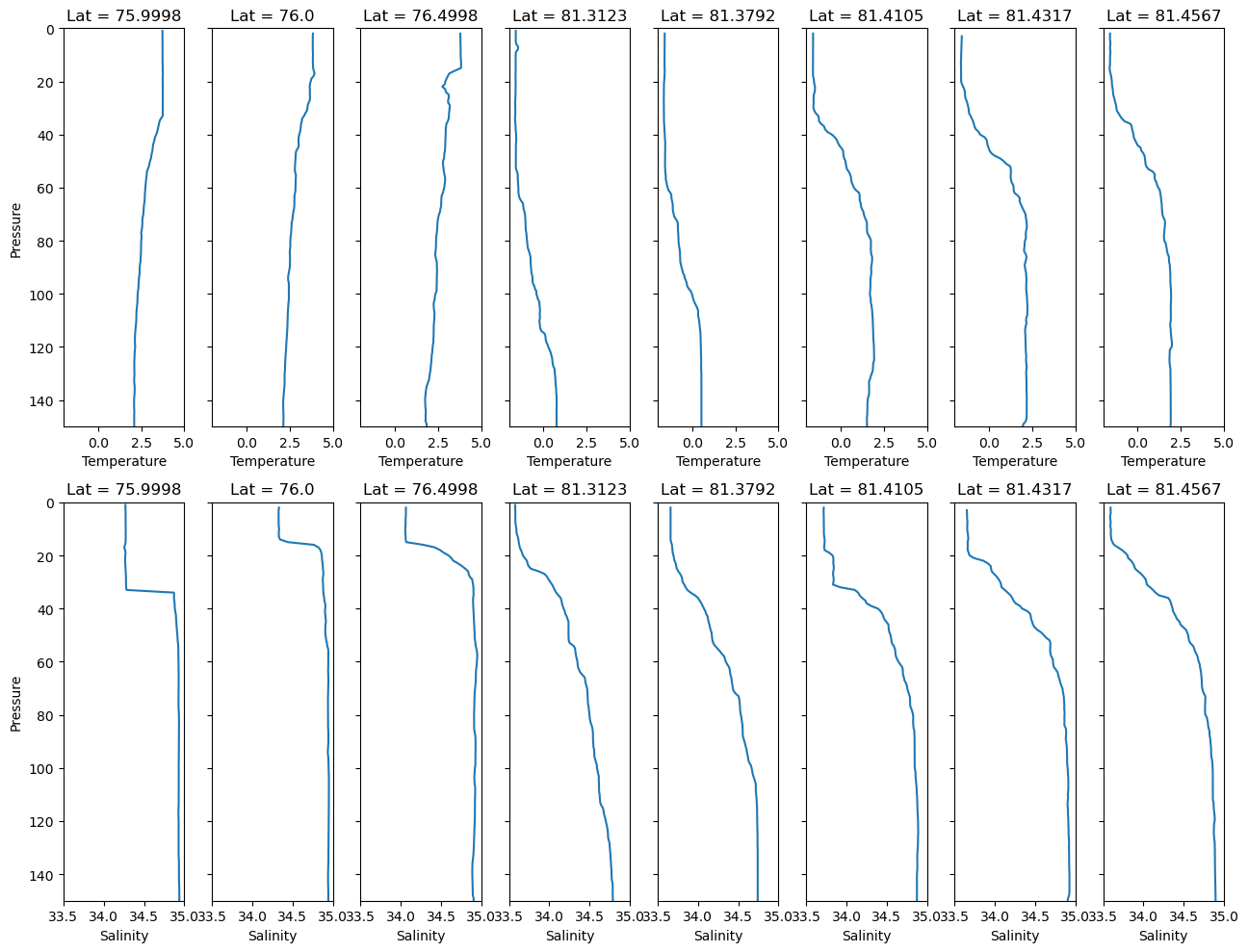
Plotting data from multiple files together

How you do this is going to depend very much on the data and your requirements. However, this is a demonstration that it is possible to create a single plot of data from multiple NetCDF files.

import matplotlib.pyplot as plt
import xarray as xr

fig, axs = plt.subplots(2, len(filtered_datasets), figsize=(13, 10), sharey=True)

# Sorting the datasets in order of latitude
sorted_latitudes = sorted(filtered_datasets.keys())

for i, latitude in enumerate(sorted_latitudes):
    xrds = filtered_datasets[latitude]
    pressure = xrds['PRES']
    temperature = xrds['TEMP']
    salinity = xrds['PSAL']

    axs[0,i].plot(temperature, pressure)
    axs[0,i].set_title(f'Lat = {latitude}')
    axs[0,i].set_ylim([150,0])
    axs[0,i].set_xlim([-2,5])
    axs[0,i].set_xlabel('Temperature')
    if i == 0:
        axs[0,i].set_ylabel('Pressure')

    axs[1,i].plot(salinity, pressure)
    axs[1,i].set_title(f'Lat = {latitude}')
    axs[1,i].set_ylim([150,0])
    axs[1,i].set_xlim([33.5,35])
    axs[1,i].set_xlabel('Salinity')
    if i == 0:
        axs[1,i].set_ylabel('Pressure')

plt.tight_layout()
plt.show()